Mar Casado PCA Validation

The aim of this document is to validate results of the ml.js package PCA method in JavaScript for an Observable course on Data Science Workflows in JavaScript (Session 3). This example closely follows the example from the palmerpenguins package documentation.

Data source: Marcos Gonçalves da Silva, Juliana Nascimento Silva, Helena Rodrigues Fragoso, Natalia Pirani Ghilardi-Lopes (2019).Temporal series analysis of abiotic data for a subtropical Brazilian rocky shore. Data in Brief, Volume 24. ISSN 2352-3409, https://doi.org/10.1016/j.dib.2019.103873.

Attach packages

library(corrr)
library(GGally)
library(recipes)
library(tidytext)
library(tidyverse)
library(lubridate)

Get data

Read in the CSV, and add a column indicating “hot moist” and “cool dry” seasons according to authors.

mc <- read_csv("marCasadoData.csv") |> 
  mutate(season = dplyr::case_when(lubridate::month(month) %in% c(10, 11, 12, 1, 2, 3) ~ "hot moist", TRUE ~ "cool dry"))

Explore correlations:

marCasadoCorr <-  mc %>%
  dplyr::select(-month, -season) %>%
  correlate() %>%
  rearrange()

Make the PCA recipe:

mc_recipe <-
  recipe(~., data = mc) %>% 
  update_role(month, season, new_role = "id") %>% 
  step_normalize(all_predictors()) %>%
  step_pca(all_predictors(), id = "pca") %>% 
  prep()

Do PCA:

mcPCA <- 
  mc_recipe %>% 
  tidy(id = "pca") 

Create a table of loadings:

mcPCA |> select(-id) |> pivot_wider(id_cols = "terms", names_from = "component", values_from = "value")

# A tibble: 9 × 10
  terms              PC1      PC2     PC3     PC4     PC5     PC6    PC7     PC8
  <chr>            <dbl>    <dbl>   <dbl>   <dbl>   <dbl>   <dbl>  <dbl>   <dbl>
1 meanHumidity  -1.93e-2 -0.186   -0.594  -0.438   0.387   0.223  -0.281  0.215 
2 meanPressure  -5.32e-1  0.112    0.213   0.0817  0.0962 -0.0950 -0.139 -0.409 
3 windSpeed     -6.08e-2  0.546   -0.441   0.0640  0.204   0.115   0.620 -0.241 
4 windDirection -3.12e-1 -0.498    0.141  -0.0771 -0.130   0.664   0.401 -0.0812
5 PAR            5.24e-1 -0.150   -0.0363  0.0385 -0.337  -0.0758  0.373  0.138 
6 seaSurfaceTe…  5.27e-1 -0.114    0.0661 -0.151   0.163   0.168  -0.174 -0.769 
7 maxTide       -3.46e-4 -0.00917 -0.448   0.672  -0.337   0.308  -0.361 -0.0934
8 minTide       -5.03e-2  0.466    0.0173 -0.527  -0.628   0.256  -0.201 -0.0315
9 salinity       2.45e-1  0.391    0.425   0.195   0.365   0.541  -0.126  0.317 
# ℹ 1 more variable: PC9 <dbl>

Visualize varianced explained by PC

mc_recipe %>% 
  tidy(id = "pca", type = "variance") %>% 
  dplyr::filter(terms == "percent variance") %>% 
  ggplot(aes(x = component, y = value)) + 
  geom_col() + 
  xlim(c(0, 10)) + 
  ylab("% Total Variance") +
  theme_minimal()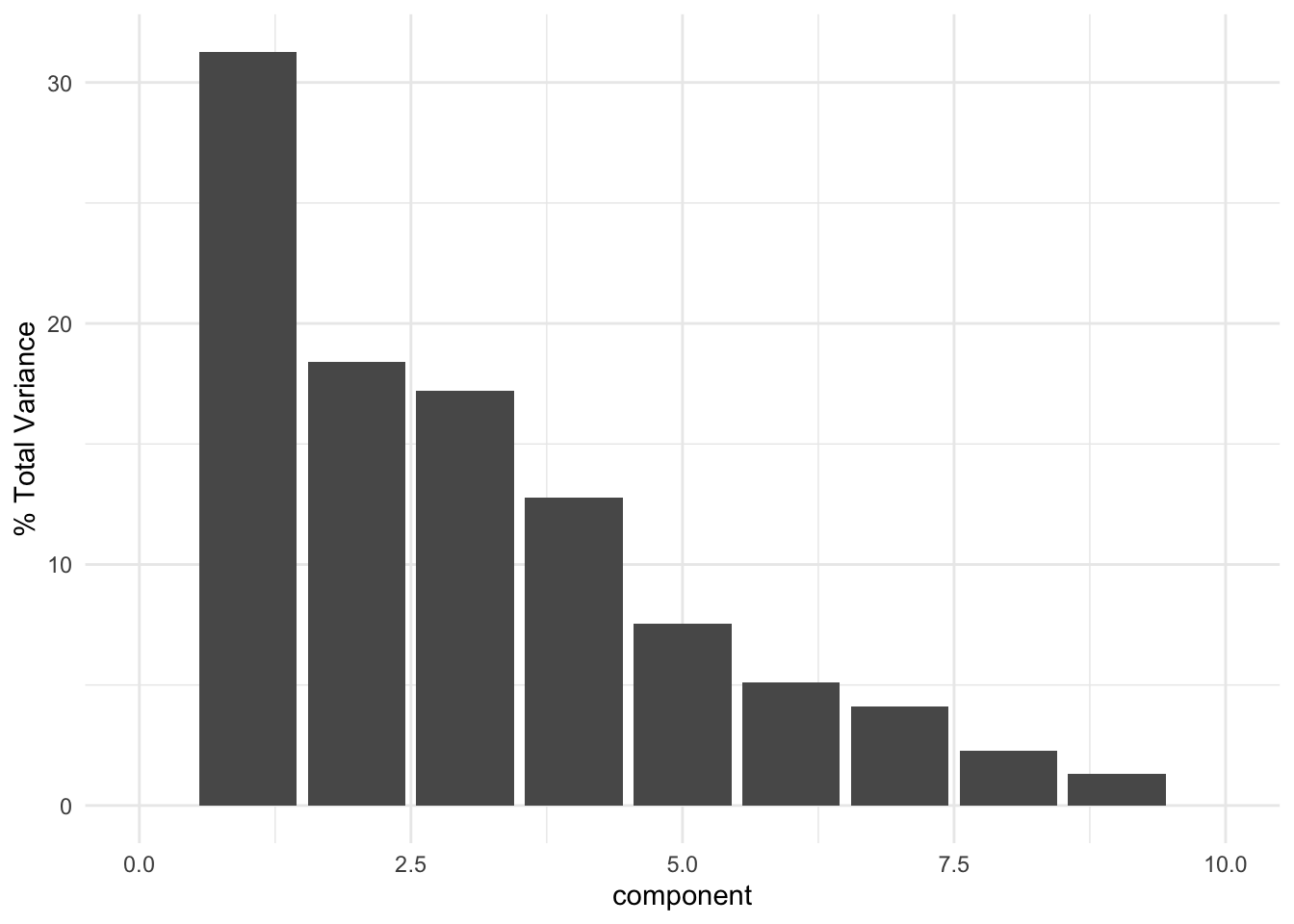

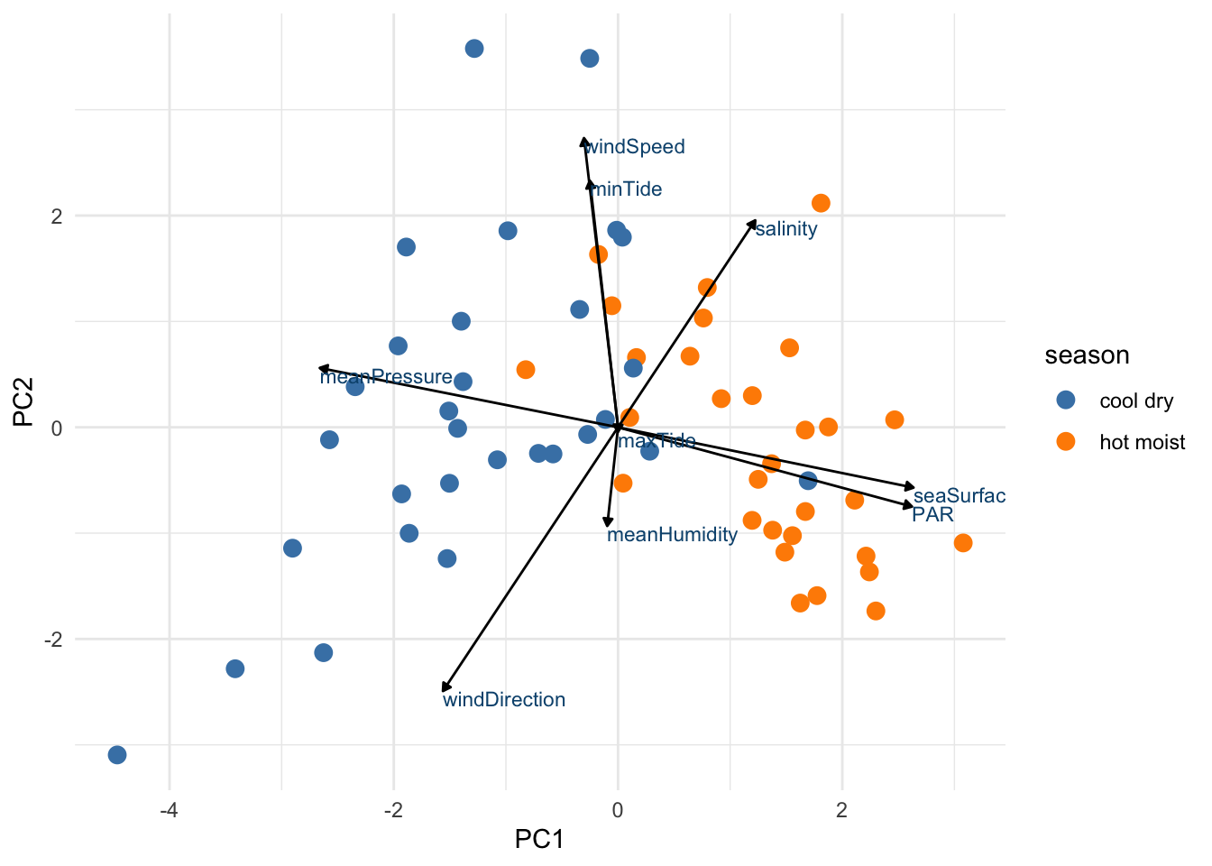
Create biplot

pca_wider <- mcPCA %>% 
  tidyr::pivot_wider(names_from = component, id_cols = terms)

arrow_style <- arrow(length = unit(.05, "inches"),
                     type = "closed")

pca_plot <-
  juice(mc_recipe) %>%
  ggplot(aes(PC1, PC2)) +
  geom_point(alpha = 1, 
             size = 3,
             aes(color = season)) + 
  scale_color_manual(values = c("steelblue", "darkorange"))

pca_plot +
  geom_segment(data = pca_wider,
               aes(xend = 5 * PC1, yend = 5 * PC2), 
               x = 0, 
               y = 0, 
               arrow = arrow_style) + 
  geom_text(data = pca_wider,
            aes(x = 5 * PC1, y = 5 * PC2, label = terms), 
            hjust = 0, 
            vjust = 1,
            size = 3, 
            color = '#0A537D') + 
  theme_minimal()