Exploring tree outcomes following fires

Author

Allison Horst

Published

March 10, 2022

Overview

Basically, there’s this awesome dataset on tree survival following fires, the Fire and Tree Mortality Database, and I want to go exploring & compare fire survival across species. Some fun with tidymodels, data visualization, binary logistic regression, and my first shot at using the fantastic geomtextpath package!

Citations:

Cansler et al. (2020). Fire and tree mortality database (FTM). Fort Collins, CO: Forest Service Research Data Archive. Updated 24 July 2020. https://doi.org/10.2737/RDS-2020-0001

Cansler et al. (2020). The Fire and Tree Mortality Database, for empirical modeling of individual tree mortality after fire. Scientific Data 7: 194. https://doi.org/10.1038/s41597-020-0522-7

Attach packages & read in the data

library(tidyverse)
library(here)
library(naniar)
library(tidymodels)
library(geomtextpath)
library(paletteer)

trees <- read_csv(here("posts", "2022-03-10-tree-mortality-fires", "data", "Data", "FTM_trees.csv")) # Tree outcomes and records

Important information: See attributes in _metadata_RDS-2020-0001.html for variable definitions.

Exploratory data visualization

Counts of tree species in the dataset:

# Find the top 20 most counted tree species
trees <- trees %>% 
  mutate(sci_name = paste(Genus, Species_name)) %>% 
  filter(sci_name != "Pinus jeffreyi or ponderosa")

tree_count_top_20 <- trees %>% 
  count(sci_name) %>% 
  mutate(sci_name = fct_reorder(sci_name, n)) %>% 
  slice_max(n, n = 20)

tree_20_gg <- ggplot(data = tree_count_top_20, aes(x = sci_name, y = n)) +
  geom_col() +
  coord_flip() +
  theme_minimal() +
  labs(y = "\nObservations in dataset",
       x = "Scientific name")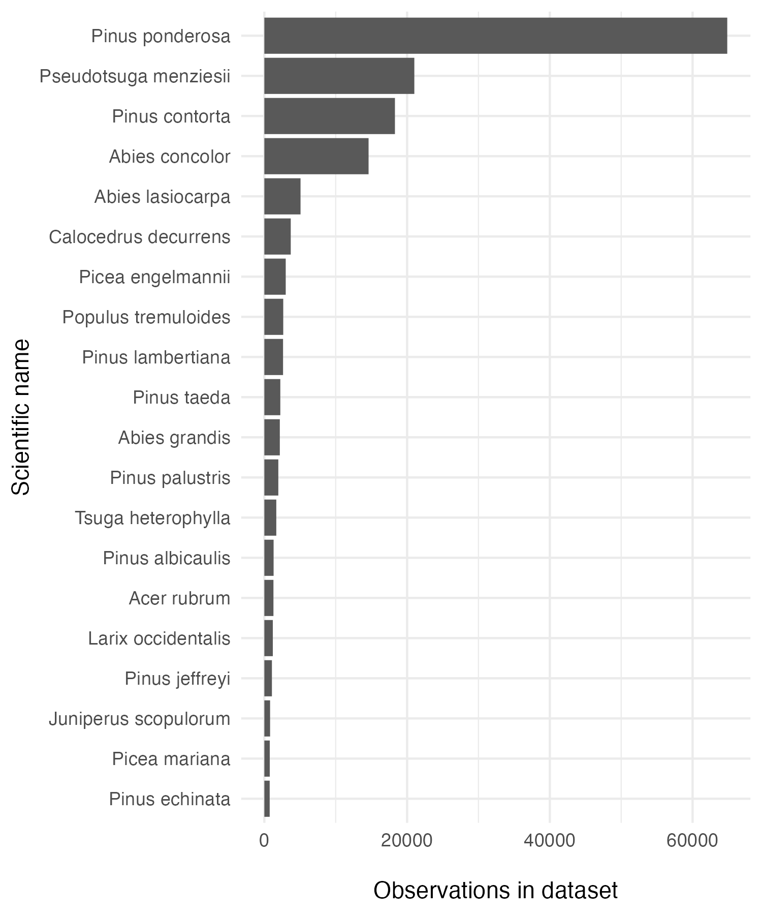

Counts of live (0) and dead (1) for the top 20 most recorded trees in the dataset:

# Make a long form of the trees dataset (top 20 most observed tree species)
trees_long <- trees %>% 
  pivot_longer(cols = yr0status:yr10status, names_to = "yr_outcome", values_to = "live_dead") %>% 
  mutate(yr_since_fire = as.numeric(parse_number(yr_outcome)),
         live_dead_chr = case_when(
           live_dead == 0 ~ "live",
           live_dead == 1 ~ "dead"
         )) %>% 
  filter(sci_name %in% tree_count_top_20$sci_name)

trees_live_dead <- trees_long %>% 
  count(sci_name, yr_since_fire, live_dead_chr) %>% 
  drop_na()
  
tree_survival_gg <- ggplot(data = trees_live_dead, aes(x = yr_since_fire, y = n)) +
  geom_col(aes(fill = live_dead_chr), position = "fill") +
  scale_fill_manual(values = c("lightsalmon", "forestgreen"),
                    name = "Live / dead:") +
  scale_x_continuous(breaks = c(0, 5, 10), labels = c("0", "5", "10")) +
  theme_minimal() +
  labs(x = "Years since fire",
       y = "Proportion live / dead",
       title = "Tree survival post-fire",
       subtitle = "Only includes the 20 most observed trees in the dataset",
       caption = "Data: Fire and tree mortality database (FTM)") +
  facet_wrap(~sci_name)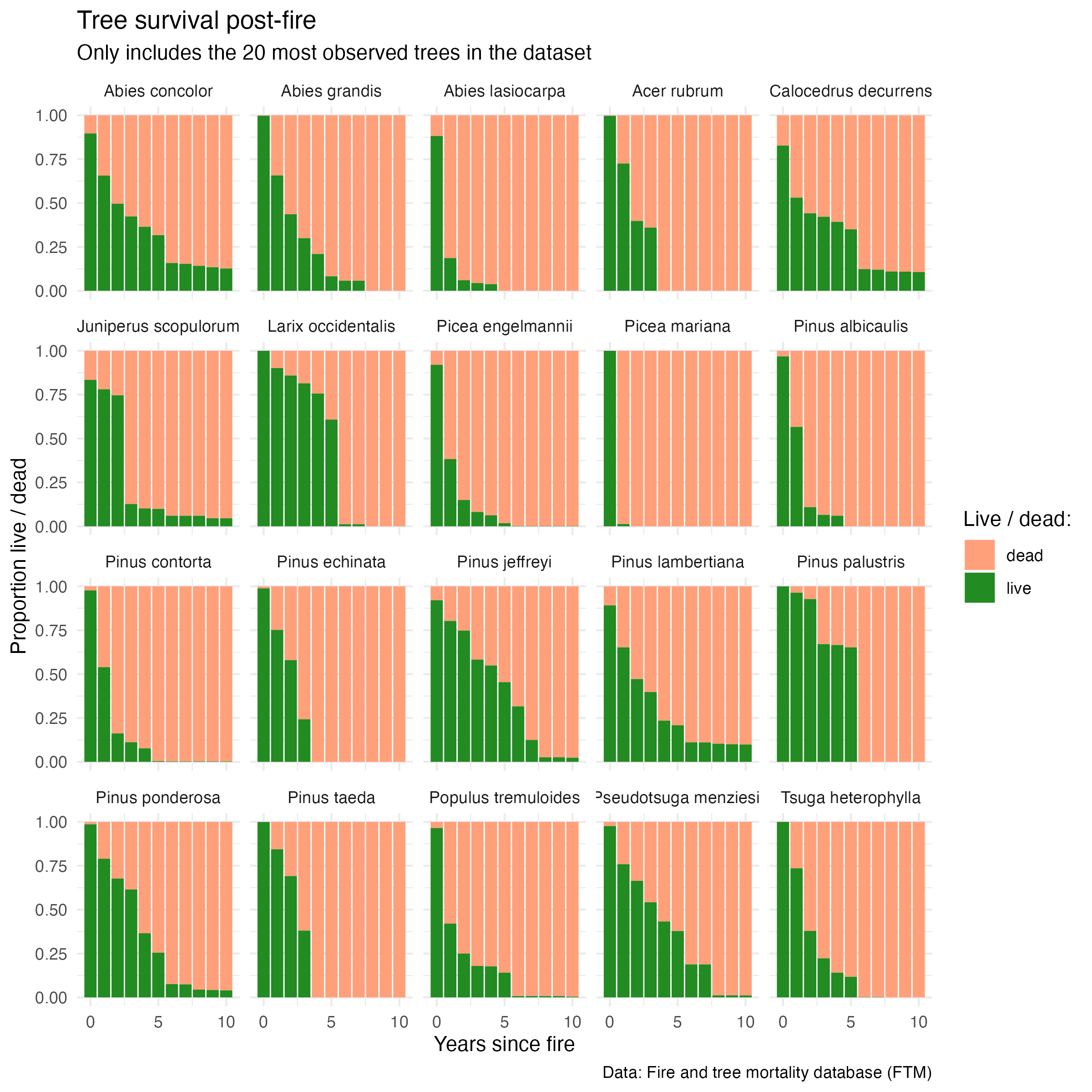

We can already see some interesting differences in survival across species. For example, Picea mariana and Abies lasiocarpa experience quick mortality within the first year; others like Pinus jeffreyi and Abies concolor appear more resilient. However, near-complete mortality is observed across all species within 10 years.

Ponderosa pines - diving a bit deeper

Since it is the most observed species in the dataset and because it happens to be one of my favorite trees, I’ll dive a bit deeper into factors that may influence Pinus ponderosa mortality post-fire.

ponderosa <- trees_long %>% 
  filter(sci_name == "Pinus ponderosa")

# write_csv(ponderosa, here::here("content", "post", "2022-03-10-tree-mortality-fires", "ponderosa.csv"))

First, let’s take a look at mortality over time (years since fire):

survival_gg <- ggplot(data = ponderosa, aes(x = yr_since_fire, y = live_dead)) +
  geom_jitter(alpha = 0.008) +
  labs(x = "Years since fire",
       y = "Tree status (live / dead)",
       title = "Ponderosa pine mortality post-fire",
       caption = "Data: Fire and tree mortality database (FTM)") +
  scale_y_continuous(breaks = c(0, 1), labels = c("Live", "Dead")) +
  scale_x_continuous(breaks = c(0, 5, 10), labels = c("0", "5", "10")) +
  theme_minimal()

Classification: binary logistic regression in `tidymodels`

Create the training & testing sets

ponderosa <- ponderosa %>% 
  drop_na(yr_since_fire, live_dead) %>% 
  mutate(live_dead = as.factor(live_dead))

# Make the training & testing dataset:
ponderosa_split <- ponderosa %>% 
  initial_split(prop = 4/5)

# Confirm the splits (Analysis/Assess/Total): 
ponderosa_split

<Training/Testing/Total>
<293297/73325/366622>

# Extract the training and testing sets: 
ponderosa_train <- training(ponderosa_split)
ponderosa_test <- testing(ponderosa_split)

# Check them out a bit: 
ponderosa_train %>% 
  count(yr_since_fire, live_dead)

# A tibble: 22 × 3
   yr_since_fire live_dead     n
           <dbl> <fct>     <int>
 1             0 0         39823
 2             0 1           566
 3             1 0         39090
 4             1 1         10394
 5             2 0         26899
 6             2 1         12947
 7             3 0         23688
 8             3 1         14719
 9             4 0          8558
10             4 1         14936
# ℹ 12 more rows

ponderosa_test %>% 
  count(yr_since_fire, live_dead)

# A tibble: 22 × 3
   yr_since_fire live_dead     n
           <dbl> <fct>     <int>
 1             0 0          9846
 2             0 1           123
 3             1 0          9789
 4             1 1          2575
 5             2 0          6809
 6             2 1          3147
 7             3 0          5865
 8             3 1          3782
 9             4 0          2245
10             4 1          3817
# ℹ 12 more rows

Make a recipe

# Just using the single predictor here:
ponderosa_recipe <- recipe(live_dead ~ yr_since_fire, data = ponderosa)
ponderosa_recipe

Make the model

ponderosa_model <- 
  logistic_reg() %>%
  set_engine("glm") %>%
  set_mode("classification") # Binary classificiation

Make the workflow

ponderosa_wf <- workflow() %>% 
  add_recipe(ponderosa_recipe) %>% 
  add_model(ponderosa_model)

Fit the model:

ponderosa_fit <- ponderosa_wf %>% 
  last_fit(ponderosa_split)

# Which returns high accuracy and roc_auc:
ponderosa_fit %>% collect_metrics()

# A tibble: 2 × 4
  .metric  .estimator .estimate .config             
  <chr>    <chr>          <dbl> <chr>               
1 accuracy binary         0.805 Preprocessor1_Model1
2 roc_auc  binary         0.879 Preprocessor1_Model1

Proof of concept: check out the test set predictions

…just for the first 20 rows:

ponderosa_fit %>% 
  collect_predictions() %>% 
  head(20)

# A tibble: 20 × 7
   id               .pred_0 .pred_1  .row .pred_class live_dead .config         
   <chr>              <dbl>   <dbl> <int> <fct>       <fct>     <chr>           
 1 train/test split  0.838   0.162      1 0           1         Preprocessor1_M…
 2 train/test split  0.912   0.0880    11 0           0         Preprocessor1_M…
 3 train/test split  0.394   0.606     18 1           1         Preprocessor1_M…
 4 train/test split  0.140   0.860     20 1           1         Preprocessor1_M…
 5 train/test split  0.140   0.860     34 1           1         Preprocessor1_M…
 6 train/test split  0.0756  0.924     35 1           1         Preprocessor1_M…
 7 train/test split  0.838   0.162     40 0           0         Preprocessor1_M…
 8 train/test split  0.912   0.0880    43 0           0         Preprocessor1_M…
 9 train/test split  0.838   0.162     48 0           0         Preprocessor1_M…
10 train/test split  0.722   0.278     52 0           1         Preprocessor1_M…
11 train/test split  0.394   0.606     54 1           1         Preprocessor1_M…
12 train/test split  0.838   0.162     62 0           0         Preprocessor1_M…
13 train/test split  0.722   0.278     67 0           0         Preprocessor1_M…
14 train/test split  0.565   0.435     68 0           1         Preprocessor1_M…
15 train/test split  0.246   0.754     70 1           1         Preprocessor1_M…
16 train/test split  0.140   0.860     71 1           1         Preprocessor1_M…
17 train/test split  0.0393  0.961     73 1           1         Preprocessor1_M…
18 train/test split  0.0201  0.980     74 1           1         Preprocessor1_M…
19 train/test split  0.838   0.162     77 0           0         Preprocessor1_M…
20 train/test split  0.722   0.278     78 0           0         Preprocessor1_M…

Confusion matrix of truth / predictions

Recall here: 0 = “Live”, 1 = “Dead”

ponderosa_fit %>% 
  collect_predictions() %>% 
  conf_mat(truth = live_dead, estimate = .pred_class)

          Truth
Prediction     0     1
         0 32309  9627
         1  4672 26717

Fit on entire dataset

ponderosa_model_full <- fit(ponderosa_wf, ponderosa)

ponderosa_model_full

══ Workflow [trained] ══════════════════════════════════════════════════════════
Preprocessor: Recipe
Model: logistic_reg()

── Preprocessor ────────────────────────────────────────────────────────────────
0 Recipe Steps

── Model ───────────────────────────────────────────────────────────────────────

Call:  stats::glm(formula = ..y ~ ., family = stats::binomial, data = data)

Coefficients:
  (Intercept)  yr_since_fire  
      -2.3424         0.6929  

Degrees of Freedom: 366621 Total (i.e. Null);  366620 Residual
Null Deviance:      508200 
Residual Deviance: 318000   AIC: 318000

Making new predictions

Let’s say we want to predict survival of other ponderosa pines based solely on years post-fire:

# Make a data frame containing a "yr_since_fire" variable as a new model input:
new_yr <- data.frame(yr_since_fire = c(0, 0.4, 1, 2.2, 5.7, 8.3))

# Then use the model to predict outcomes, bind together: 
example_predictions <- data.frame(new_yr, predict(ponderosa_model_full, new_yr))

example_predictions

  yr_since_fire .pred_class
1           0.0           0
2           0.4           0
3           1.0           0
4           2.2           0
5           5.7           1
6           8.3           1

This does seem to align with what we’d expect based on the data visualization. We can also find the probability of “Dead” (outcome = 1) using the model predictions, adding type = "prob" within the predict() function.

predict_over <- data.frame(yr_since_fire = seq(from = 0, to = 10, by = 0.1))
predictions_full <- data.frame(predict_over, predict(ponderosa_model_full, predict_over, type = "prob"))
names(predictions_full) <- c("yr_since_fire", "prob_alive", "prob_dead")

# Plot probability of mortality:
ponderosa_prob_alive <- ggplot() +
  geom_line(data = predictions_full, aes(x = yr_since_fire, y = prob_alive), color = "gray30", size = 1) +
  labs(x = "Years since fire",
       y = "Probability of tree being alive",
       title = "Predicted Ponderosa pine mortality post-fire",
       caption = "Data: Fire and tree mortality database (FTM)") +
  scale_y_continuous(breaks = c(0, 0.5,  1), 
                     labels = c("0%", "50%", "100%"),
                     limits = c(0, 1)) +
  scale_x_continuous(breaks = c(0, 5, 10), labels = c("0", "5", "10")) +
  theme_minimal()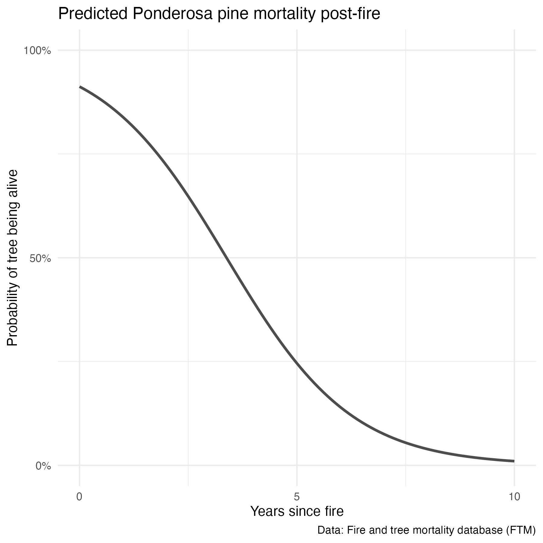

Extending the model

I want to extend this model for the 20 most observed trees in the dataset (so will include species as a predictor variable).

Create the training & testing sets

trees_20 <- trees_long %>% 
  filter(sci_name %in% c(tree_count_top_20$sci_name)) %>% 
  drop_na(yr_since_fire, live_dead) %>% 
  mutate(live_dead = as.factor(live_dead))

# Make the training & testing dataset:
trees_20_split <- trees_20 %>% 
  initial_split(prop = 4/5)

# Confirm the splits (Analysis/Assess/Total): 
trees_20_split

<Training/Testing/Total>
<830790/207698/1038488>

# Extract the training and testing sets: 
trees_20_train <- training(trees_20_split)
trees_20_test <- testing(trees_20_split)

# Check them out a bit: 
trees_20_train %>% 
  count(yr_since_fire, live_dead)

# A tibble: 22 × 3
   yr_since_fire live_dead     n
           <dbl> <fct>     <int>
 1             0 0         77750
 2             0 1          2951
 3             1 0         73690
 4             1 1         30565
 5             2 0         51605
 6             2 1         47263
 7             3 0         43212
 8             3 1         54768
 9             4 0         22517
10             4 1         55525
# ℹ 12 more rows

trees_20_test %>% 
  count(yr_since_fire, live_dead)

# A tibble: 22 × 3
   yr_since_fire live_dead     n
           <dbl> <fct>     <int>
 1             0 0         19376
 2             0 1           703
 3             1 0         18073
 4             1 1          7629
 5             2 0         12931
 6             2 1         11803
 7             3 0         10749
 8             3 1         13700
 9             4 0          5509
10             4 1         13918
# ℹ 12 more rows

Make a recipe

# Just using the single predictor here:
trees_20_recipe <- recipe(live_dead ~ yr_since_fire + sci_name, data = trees_20)
trees_20_recipe

Make the model

trees_20_model <- 
  logistic_reg() %>%
  set_engine("glm") %>%
  set_mode("classification") # Binary classificiation

Make the workflow

trees_20_wf <- workflow() %>% 
  add_recipe(trees_20_recipe) %>% 
  add_model(trees_20_model)

Fit the model:

trees_20_fit <- trees_20_wf %>% 
  last_fit(trees_20_split)

# Which returns high accuracy and roc_auc:
trees_20_fit %>% collect_metrics()

# A tibble: 2 × 4
  .metric  .estimator .estimate .config             
  <chr>    <chr>          <dbl> <chr>               
1 accuracy binary         0.820 Preprocessor1_Model1
2 roc_auc  binary         0.893 Preprocessor1_Model1

Confusion matrix of truth / predictions

Recall here: 0 = “Live”, 1 = “Dead”

trees_20_fit %>% 
  collect_predictions() %>% 
  conf_mat(truth = live_dead, estimate = .pred_class)

          Truth
Prediction      0      1
         0  57085  19977
         1  17376 113260

Fit on entire dataset

trees_20_model_full <- fit(trees_20_wf, trees_20)

trees_20_model_full

══ Workflow [trained] ══════════════════════════════════════════════════════════
Preprocessor: Recipe
Model: logistic_reg()

── Preprocessor ────────────────────────────────────────────────────────────────
0 Recipe Steps

── Model ───────────────────────────────────────────────────────────────────────

Call:  stats::glm(formula = ..y ~ ., family = stats::binomial, data = data)

Coefficients:
                  (Intercept)                  yr_since_fire  
                     -1.89320                        0.61524  
        sci_nameAbies grandis       sci_nameAbies lasiocarpa  
                      0.69818                        2.72269  
          sci_nameAcer rubrum   sci_nameCalocedrus decurrens  
                      0.54265                        0.24419  
 sci_nameJuniperus scopulorum     sci_nameLarix occidentalis  
                      0.94475                       -1.21916  
    sci_namePicea engelmannii          sci_namePicea mariana  
                      1.88703                        5.68710  
     sci_namePinus albicaulis         sci_namePinus contorta  
                      2.17161                        1.78648  
       sci_namePinus echinata         sci_namePinus jeffreyi  
                      0.56136                       -0.54492  
    sci_namePinus lambertiana        sci_namePinus palustris  
                      0.30286                       -1.42278  
      sci_namePinus ponderosa            sci_namePinus taeda  
                     -0.21649                        0.06294  
  sci_namePopulus tremuloides  sci_namePseudotsuga menziesii  
                      1.30545                       -0.27530  
   sci_nameTsuga heterophylla  
                      0.82540  

Degrees of Freedom: 1038487 Total (i.e. Null);  1038467 Residual
Null Deviance:      1358000 
Residual Deviance: 818700   AIC: 818700

Mortality (probability)

# Make a data frame containing a "sci_name" and "yr_since_fire" variable as a new model input:
new_data <- data.frame(sci_name = rep(unique(trees_20$sci_name), 100)) %>% 
  arrange(sci_name)

new_data <- data.frame(new_data, yr_since_fire = rep(seq(from = 0, to = 10, length = 100), 20))

tree_20_predictions <- data.frame(new_data, predict(trees_20_model_full, new_data, type = "prob"))
names(tree_20_predictions) <- c("sci_name", "yr_since_fire", "prob_alive", "prob_dead")

# Plot probability of mortality:
all_prob_gg <- ggplot() +
  geom_textline(data = tree_20_predictions, 
                aes(x = yr_since_fire, 
                    y = prob_alive, 
                    label = sci_name,
                    group = sci_name,
                    color = sci_name), 
                size = 2.5,
                show.legend = FALSE) +
  labs(x = "Years since fire",
       y = "Probability of tree being alive",
       title = "Predicted tree mortality post-fire",
       caption = "Data: Fire and tree mortality database (FTM)") +
  scale_y_continuous(breaks = c(0, 0.5,  1), 
                     labels = c("0%", "50%", "100%"),
                     limits = c(0, 1)) +
  scale_x_continuous(breaks = c(0, 5, 10), labels = c("0", "5", "10")) +
  scale_color_paletteer_d("ggthemes::Tableau_20") +
  theme_minimal()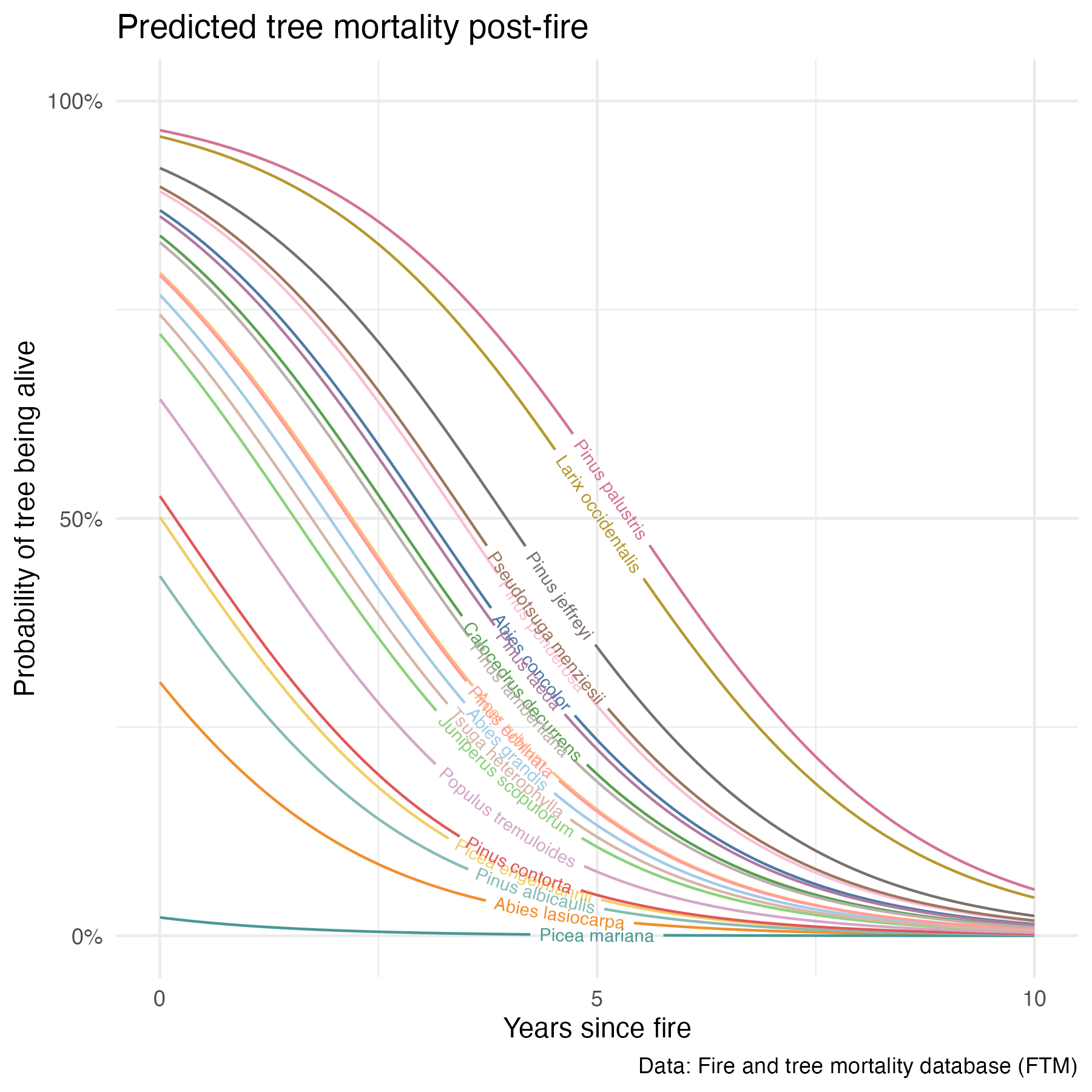

More opportunities

There are a bunch of other variables in this dataset that would be worth considering - like how scorched the tree is post-fire, how large it was to start (height and diameter), evidence of beetle infestation, and more - I’m looking forward to coming back to this dataset in the future & revisiting this model with additional investigation of those variables.

Overview

Citations:

Attach packages & read in the data

Exploratory data visualization

Ponderosa pines - diving a bit deeper

Classification: binary logistic regression in tidymodels

Make a recipe

Make the model

Make the workflow

Fit the model:

Proof of concept: check out the test set predictions

Confusion matrix of truth / predictions

Fit on entire dataset

Making new predictions

Extending the model

Make a recipe

Make the model

Make the workflow

Fit the model:

Confusion matrix of truth / predictions

Fit on entire dataset

Mortality (probability)

More opportunities

Classification: binary logistic regression in `tidymodels`